TP 2: segmentation and classification of PreTest signals
Balthazar Neveu
Topics:
- Noisy labels
- Imbalanced dataset
- Feature extraction
- Dimension reduction
Problem statement
- Total normal samples: 85 = 35.1%
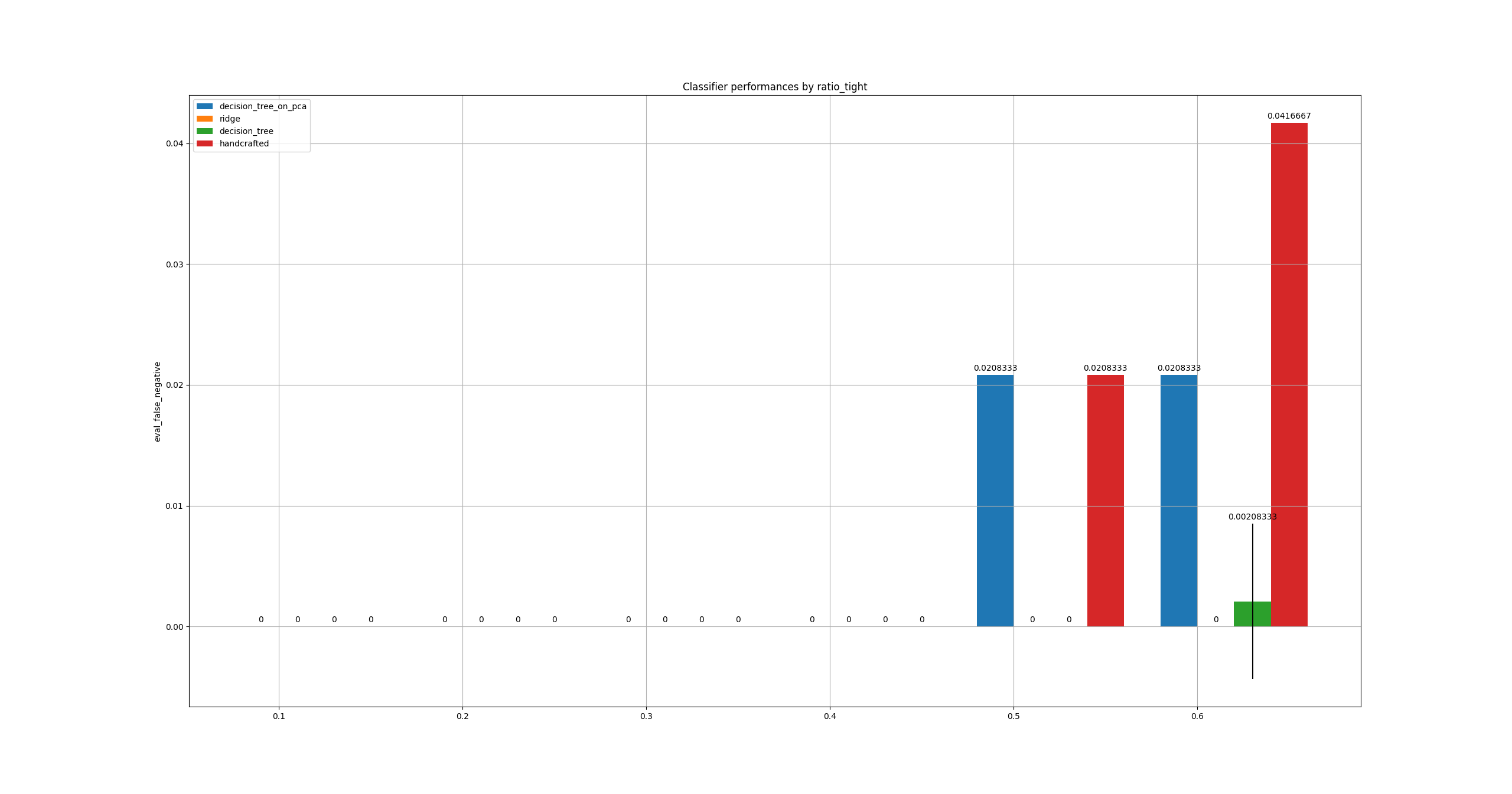
- Total tight samples: 157 = 64.9% (dominant class)
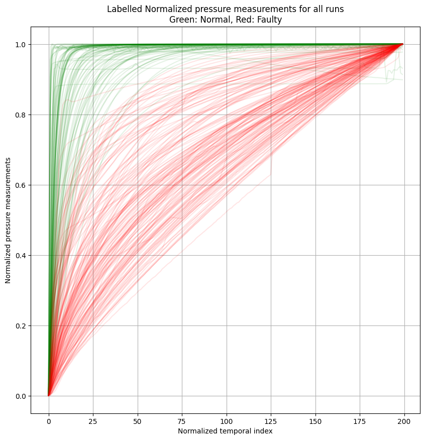
- Classify a set of pressure profiles.
- 🟢 Green: normal $\text{label}=1$
- 🔴 Red: Tight $\text{label}=0$
Exploration: Reparameterization and handcrafted features
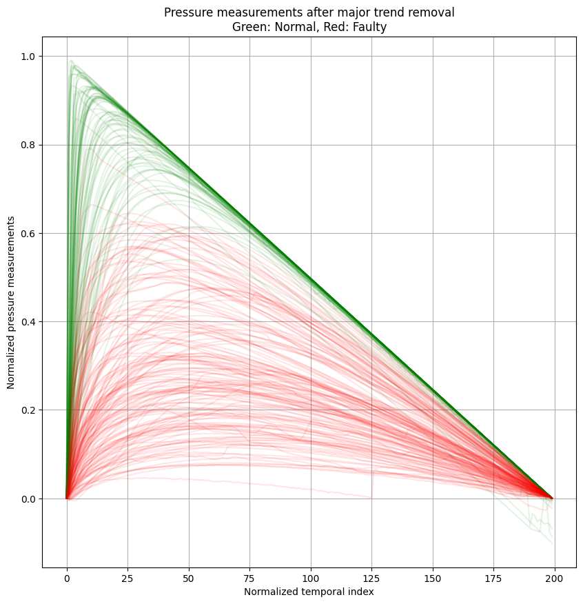
- Remove the "identity trend"
- Maximum value of these curves looks like a good discriminator.
Exploration: Handcrafted feature
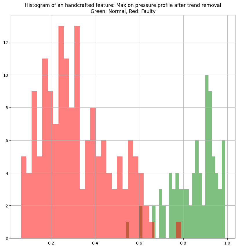
- Histogram of this handcrafted feature for the 2 labelled classes.
- A simple threshold around 0.7 could be enough to discriminate these 2 classes. Simple to compute, yet seems efficient.
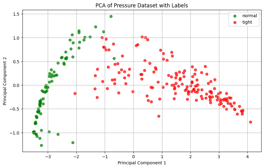
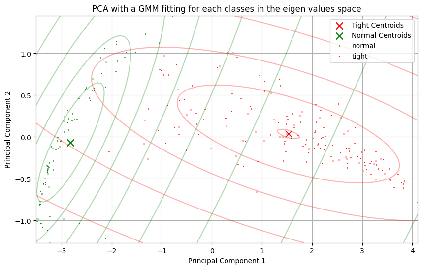
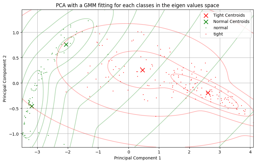
Exploration: PCA
- When we apply a principal component analyzis to the raw curves, we're able to see 2 clusters appear in the 2D eigen cofficient space.
- Each pressure curve made of 200 samples has been mapped to a single 2D vector.
- Knowing the labels, 2 obvious clusters appear.
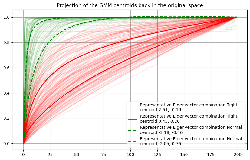
2D Gaussian Fitting
- If we reproject the centroid back into the original pressure curve space, we can see that these curves are pretty representative of the 2 distributions in the original space.
- These are simple combinations of the 2 eigenvectors.
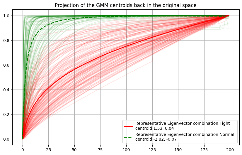
Please note that scikitlearn applies a mean centering to perform PCA
Classification
- Precision: classified a normal event as normal $\frac{tp}{tp+fp}$: classifier ability not to label as positive a sample that is negative. 💲
- Recall: classified $\frac{tp}{tp+fn}$ : the classifier ability to find all the positive samples.. We want a recall of 100% here ❌ !
- Confusion matrix: $C_{i, j}$
- $i$ groundtruth class
- $j$ predicted class
| Confusion matrix | Prediction $j=0$ Tight | Prediction $j=1$ Normal |
|---|---|---|
| Groundtruth $i=0$ Tight | True Negative (groundtruth=tight, prediction=tight) ✔️ | False Positive (groundtruth=tight,prediction=normal) 💲 |
| Groundtruth $i=1$ Normal | False Negative (groundtruth=normal, prediction=Tight) ❌ | True Positive (groundtruth=normal, prediction=normal) ✔️ |
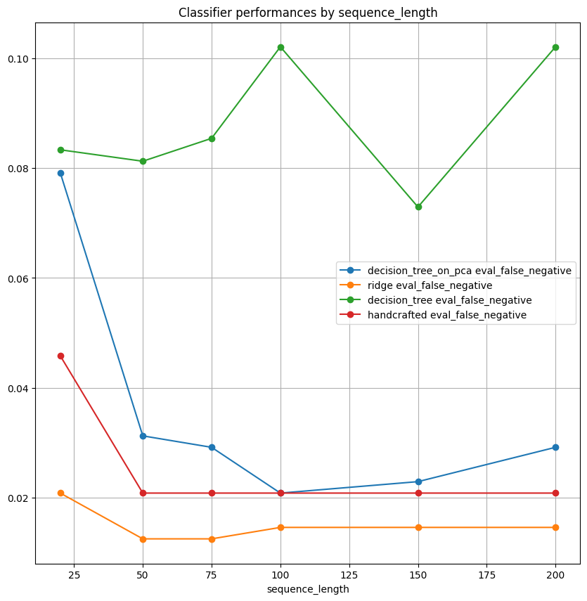
Study with regard to pressure test length
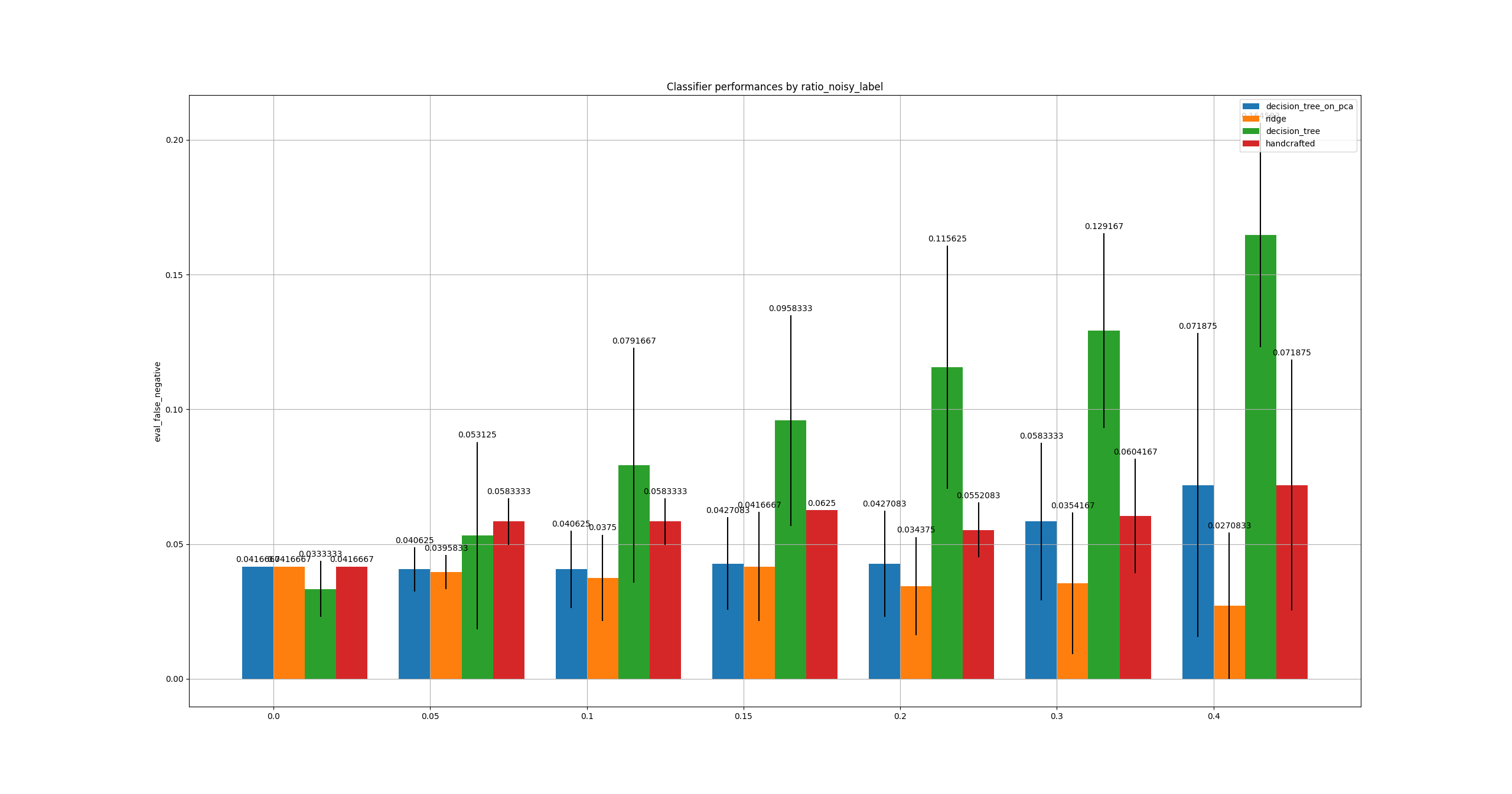
Study with regard to labelling quality
Conclusions
- Very low data regime.
- Simplicity: Handcrafted features with very basic classifier achieves quite decent results.
- False Negative is the most important metric for this topic. False Positives may increase costs.
- More work to be done to decrease and reach 0% of false positives, either by adding metadata or making more complex classifiers.
- Class imbalance does not seem to affect results too much here. Noisy labels either.
- Known method limitations:
- Cross validation is performed by sampling several noisy train sets... while test set remains the same to get a fixed test set reference without noise.
- Not using metatada
- No true way to specifically minimize false negatives.
- Quid: resampling on time dimension, did we loose information
How to use?
- Notebook
- Command line interface:
python TP_2/code/train_classifiers.py --study sequence_lengths_study_noisy -r 20- Choices of studies:
sequence_lengths_study: vary pressure test duration, perfect labels, perfect class balance (50%-50%)sequence_lengths_study_noisy: vary pressure test duration, slightly noisy labels (20%)noisy_labels_study: study the influence of the amount of noisy labels on final performances.tight_ratio: tight class ration: variation of class imbalance