Segmentation¶

Balthazar Neveu
Project= updated TP-5 for Introduction to geosciences | ENS Paris Saclay - Master MVA 2024
Web version | Github

Disclaimer¶

🆕 since I discovered some issues (mentioned later) compared to the original TP-5 version , I had to start all over again ...

I modified this technical report with some updates and mentioned it by adding the logo 🆕.

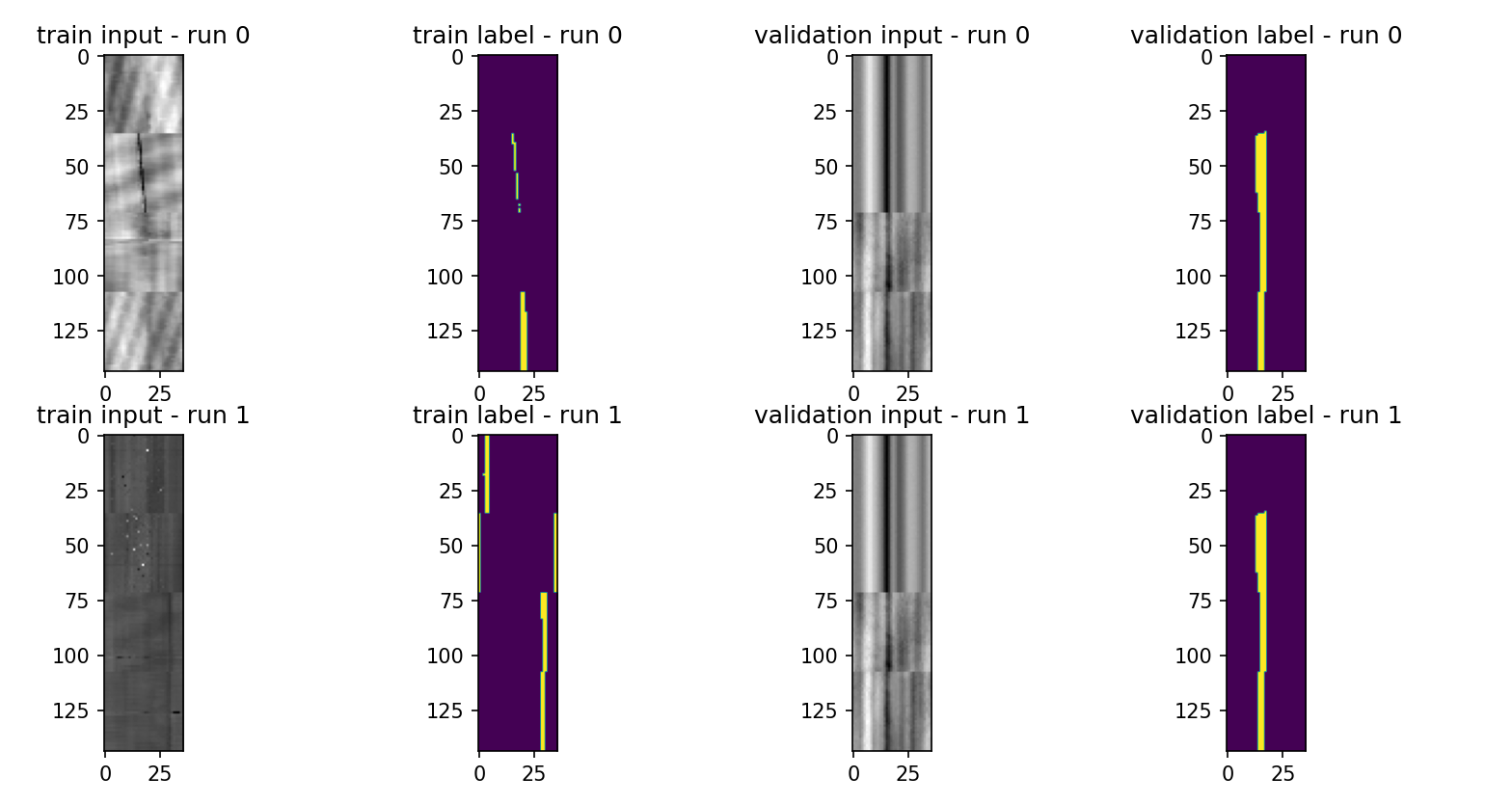
Dataset exploration¶

Pairs of patches and annotations (areas to segment). size 36x36 gray level.

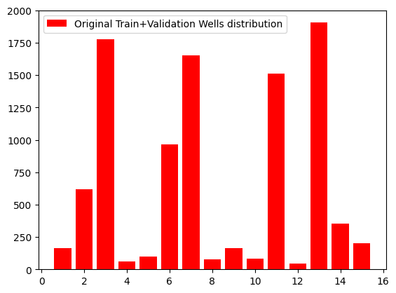
Train set: 7211 patches from 12 wells.
Validation set: 2463 patches from 3 wells (majority in well 13)

⚠️ WARNING no wells in common between validation and training ⚠️.

Observations

At first sight, the regions we're trying to segment look like thin dark lines.
Sometimes the positive areas are spread on both sides of the image (due to the circular nature of the well images).
Two images containing NaN values validation/images/well_15_patch_201.npy and well_15_patch_202.npy are discarded in the dataloader (sanity check before loading the images).

Dataloader¶

data_loader.py loads pairs of image, labels. A list of augmentations is provided in augmentations.py:

Horizontal roll (since the pipelines are circular)
Vertical/Horizontal flips can be performed randomly. Random augmentations (and shuffles) are only performed on the training set, validation set is frozen.

🆕 Revision¶

A reboot has been performed compared to the TP-5 version. Sections indicated with 🆕 show the main changes.

Several critical issues have been corrected:

❌ Problem : Metrics reduction bug
✔️ Solution: simple unit tests, code review.
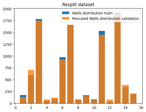
❌ Validation has not intersection with Training set. (=not the same wells)! Not a good idea to monitor training with this.
✔️ Solution: shuffle dataset (next level would be cross validation)
❌ Problem: Potential other bugs? - More generally, how to aleviate the doubts I had about the training method and architectures.
✔️ I created a toy example to validate that everything works correctly

Metrics reduction:¶

I corrected a critical bug in metrics computation (reduction must be done over batches after computing dice score/IOU/precision/recall per images) . A unitary pytest has been added.
Special case of dice score when there is no corrosion (label image = 0). If the prediction is perfect, the original formulation of the dice score gives 0%. I corrected so it is 100% to avoid penalizing. Please note that this workaround breaks the loss "continuity"... (any tiny mispredicted pixel will bring back the dice score to nearly 0%).
I also checked that metrics don't change when batch size changes...

Train/Validation gap and monitoring¶

⚠️ Although the initial idea of a validation set with wells not contained in the training set seems pretty good. It is a very deceitful idea when we're using the validation set as a metric to monitor training:

pick the best model on validation dice score ... may simply get you an overall bad model but by chance good on the 3 wells of the validation set.

LR scheduler based on this metric will reduce learning rate

Usually, we use the validation metric to monitor overfitting etc... here the validation set is way more like a "generalization to unseen data" test set.

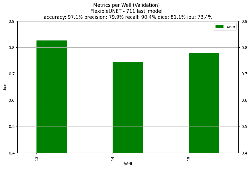
Here's what happened, I'd naturally pick the "best" model based on the validation dice score.

Performances on the "best model" according to the validation dice score	Performances at the last epoch
Train set Dice 66.2%	Train set Dice 76.5%

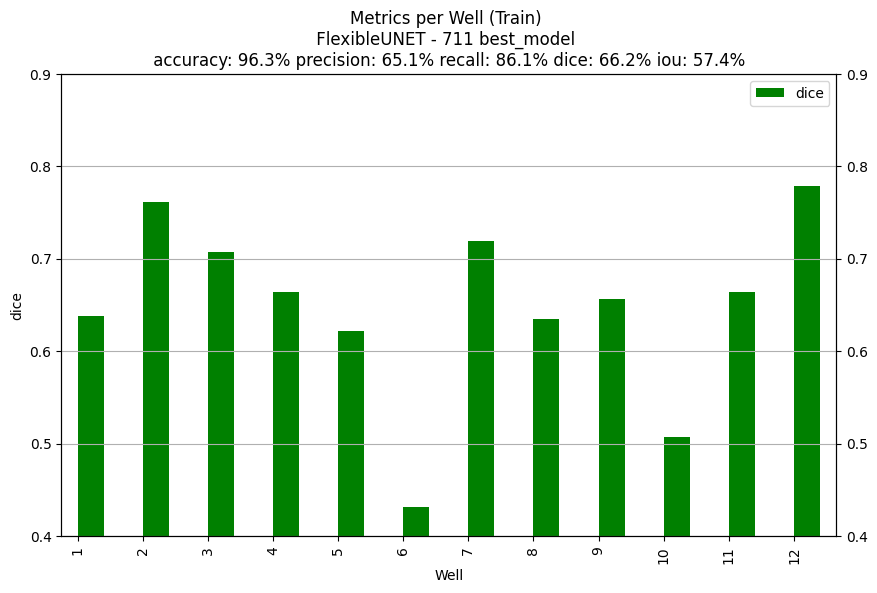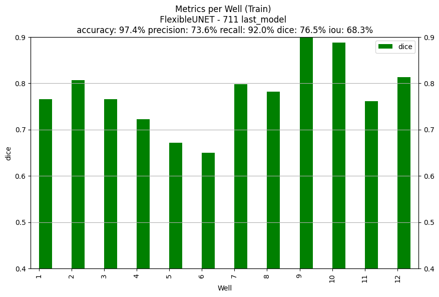Validation Dice 82.3%	Validation Dice 81.1%

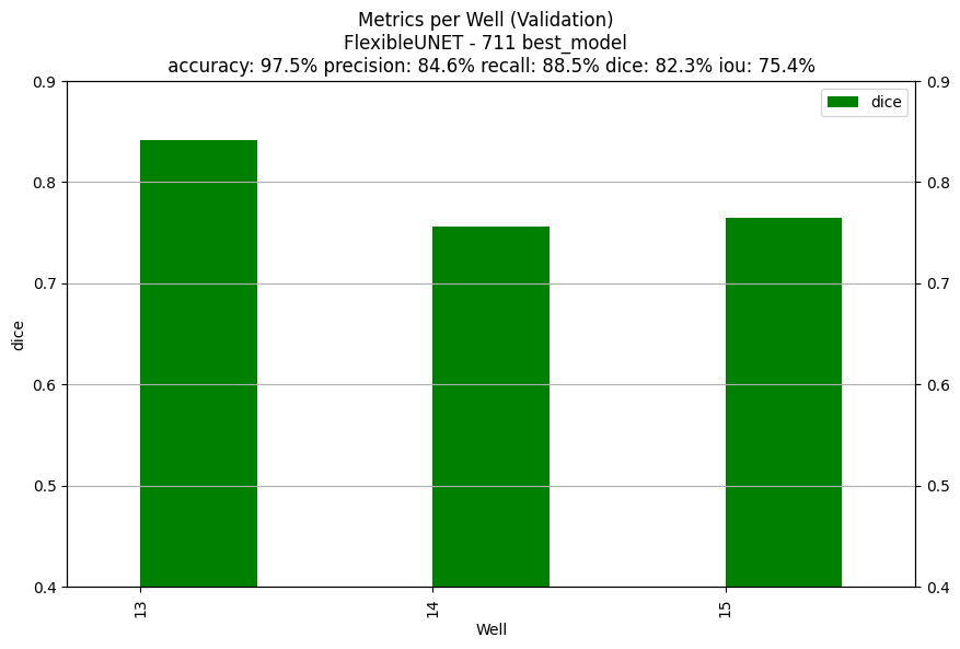Original train + validation sets wells distribution	New split distribution

🆕 Segmentation training sanity check¶

After spotting the bug in the metrics computations, I decided to check the whole pipelines for bug.

Added unit tests on metrics
Created a toy example (with various of complexity) to validate the whole training process when labels are perfect.

The toy example allows to check:

That the training loop works properly
That my models can segment perfectly labeled data properly
To check that models can be trained using the dice loss.

Exp 621 (purple) is trained using weighted BCE (x2 in favor of positive examples) and batches of size 32
Exp 622 (green) is trained in the same conditions as 621 but with batches of size 256 (which shows a slightly slower convergence)
Exp 623 (red) is trained using dice loss ... we can see that there's a drop in DICE metric at epoch 23 (but the BCE decreases).

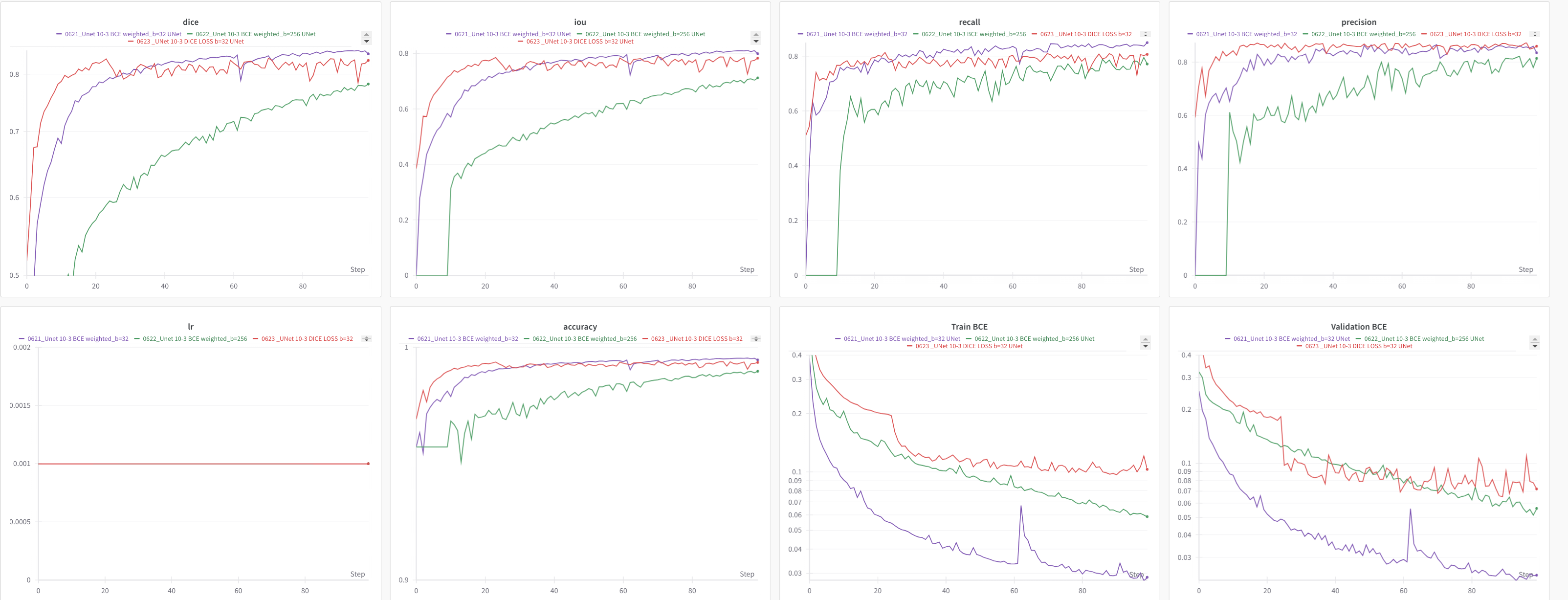Architectures¶

Three families of models are coded in different python files, access model.py to find your way All models are pretty flexible. What can be changed:

convolution sizes
number of layers
number of channels (hidden dimensions)
activation function (Relu of Leaky ReLu were tested)
number of input channels (ready to apply to other modalities)
number of output channels (ready for multi classes). Since all models inherit from BaseModel, the number of parameters and the receptive field can easily be retrieved. Please note that all models do not include the sigmoïd applied to the final layer: we take logits as outputs and the loss function or further inference is in charge of applying the sigmoïd to convert these to probabilities.

Model name	Number of parameters	Convolution sizes	Number of layers	Activation	Receptive field (H, V)
Vanilla Stacked convolutions	260k	$(3,3)$	5	ReLu	$(11,11)$
Stack convolution	1.904M	$3^{\circ} \perp 5$	5	LeakyReLu	$(11,21)$
Legacy U-Net	775k	$(3,3)$	3 scales	LeakyReLu	$(27, 27)$
🆕 Flexible U-Net Teacher	6.4M	$(3^{\circ},3)$	3 scales with 4-2-1 conv blocks	Leaky Relu	$(81,81)$
🆕 Flexible U-Net Student	576k	$(3^{\circ},3)$	3 scales with 2-1-1 conv blocks	Leaky Relu	$(73,73)$

Please note that the receptive field of the Flexible UNets are larger than the image, we avoid adding too much convolutions at the top level/bottleneck to avoid issues at boundaries and we use repeat padding to let the network think that vertically, the well goes continuously (instead of zero-ing out). For the azimuth direction, a special padding has been designed.

Vanilla convolution stack (single scale)¶

Remark: I coded the stacked convolution before I re-discovered the slide on the proposed vanilla model ("baseline" model from the slides).

Provided as a "baseline" model, uses ReLu .

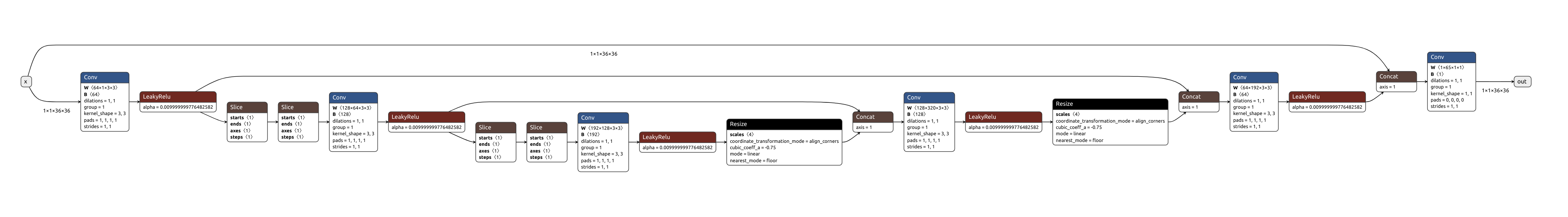
Proposed diagram by the SLB challenge organizers	Netron visualization

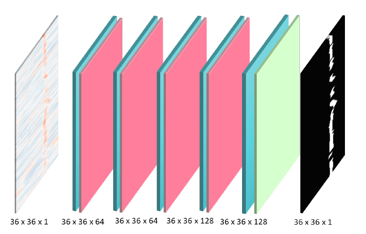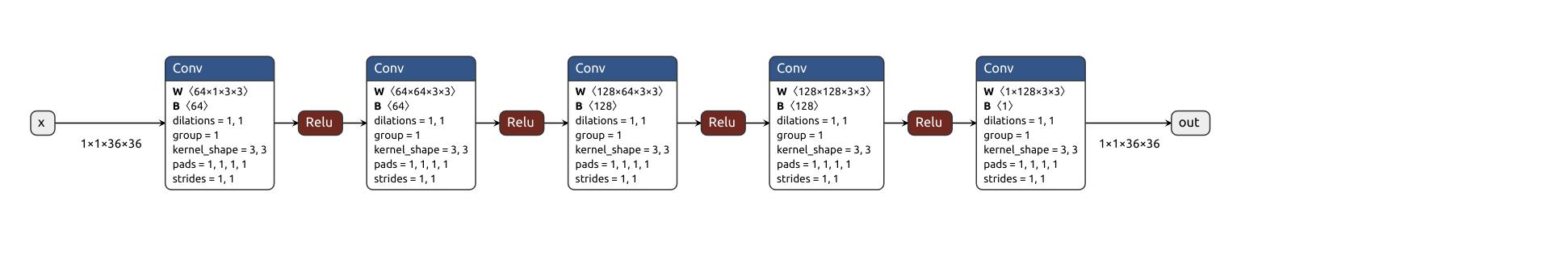Stacked convolution (single scale)¶

Flexible design with a parameterized amount of layers
Base convolution block is a separable convolution directionwise ($H \perp V$)
- The horizontal convolution pads using the "circular" convolution option which allows dealing with the specificity of dwell images.
- The vertical convolution pads by repeating gray levels.
- This should explain the notation $3^{\circ} \perp 5$
Input modality convolution block allows going from 1 to h_dim channels.
Output modality convolution block allows going from h_dim channels back to a single channel.
Last layer outputs an image of the same size as the original one. Since we use the BCE Loss with Logits at first, the output of the network are logits (not probabilities), Sigmoid is not included.
Possibility to use residual connections when the number of layers is a multiple of 2.

Legacy "Classic" UNet ¶

3 scales.
- $(36, 36) \rightarrow (18, 18) \rightarrow (9, 9)$
- Downsample by decimating information (skip 1 pixel over 4)
- Upsample with a bilinear interpolation.
- Concatenate skip connections together.
Large receptive field (27,27)

🆕 Flexible UNET ¶

After the "reboot", I decided to recode a new UNET:

pre-pad the inputs (circular padding on the azimuth direction) and crop at the end.
extend the channels dimension by a factor of 2 when downsampling, shrink the channels by 2 when upsampling.
Allow to specify:
- the amount of convolution blocks per scale for both encoder and decoder (and bottleneck)
- the thickness (width) used at the first scale... the rest is deduced progressively (using the rule x2 when downsampling by 2)

During the padding phase, we repeat a few pixels at the top and bottom (to go to a size of 40 instead of 36 which allows adding a potential 4th scale - this was not retained as the best model though and allows increasing the receptive field).

Padding mechanism for the flexible circular UNet

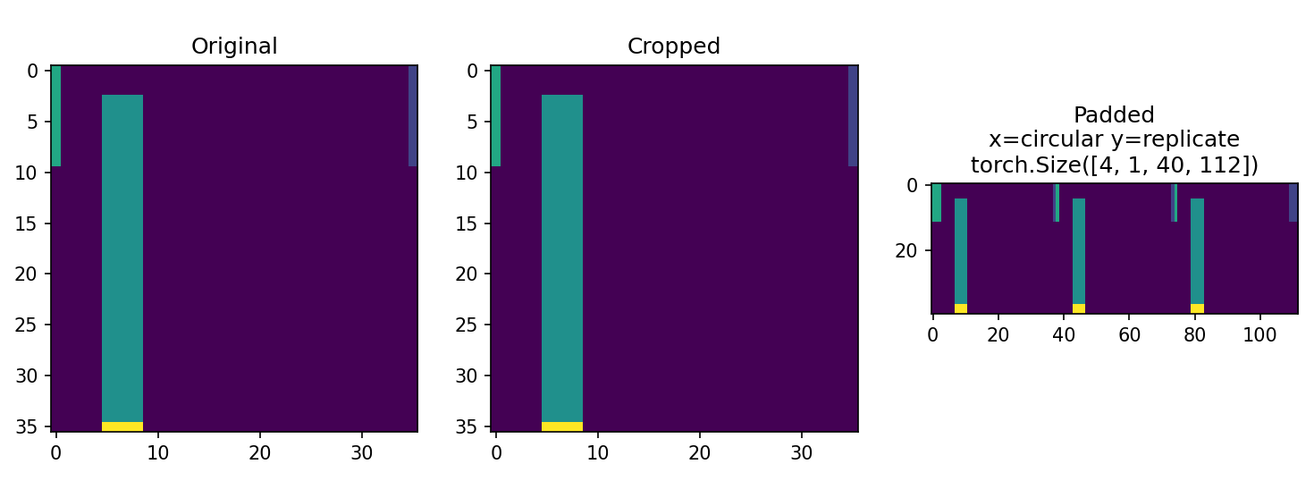Syntax for the encoder / bottleneck / decoder goes as follows: [4 , 2, 1], 1, [1, 2, 4 ] and the convolution block Thickness. It allows easily playing with the architecture.

Exp id	Dice Validation	Encoder	Bottlneck	Decoder	Thickness	# params
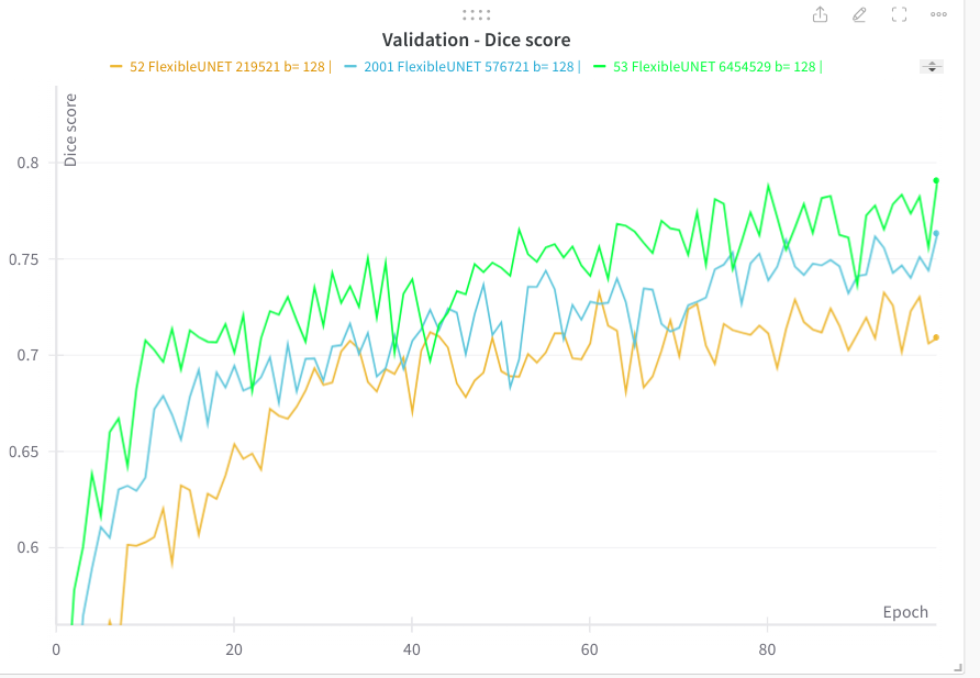
53	79%	[4, 2, 1]	1	[1, 2, 4]	64	6.4M params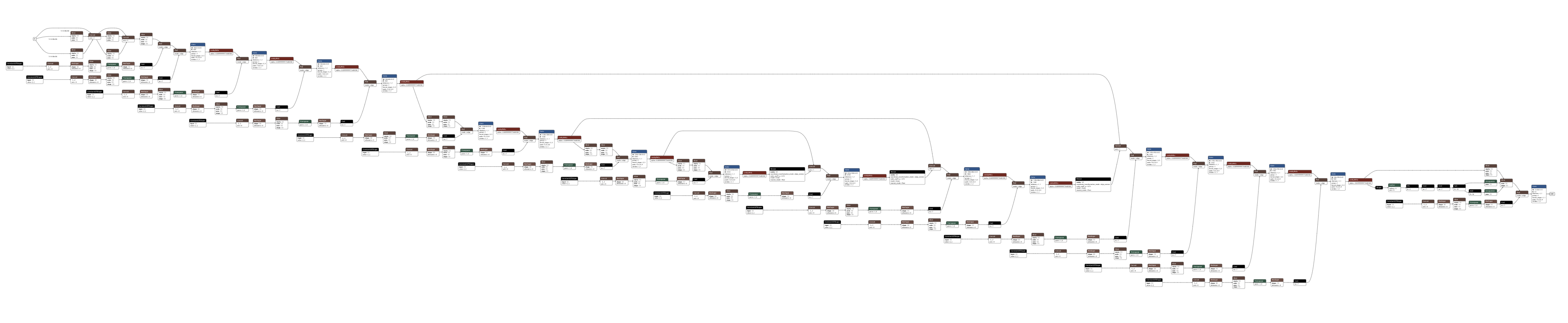
2001	76%	[4, 2, 1]	1	[1, 2, 4]	16	576k params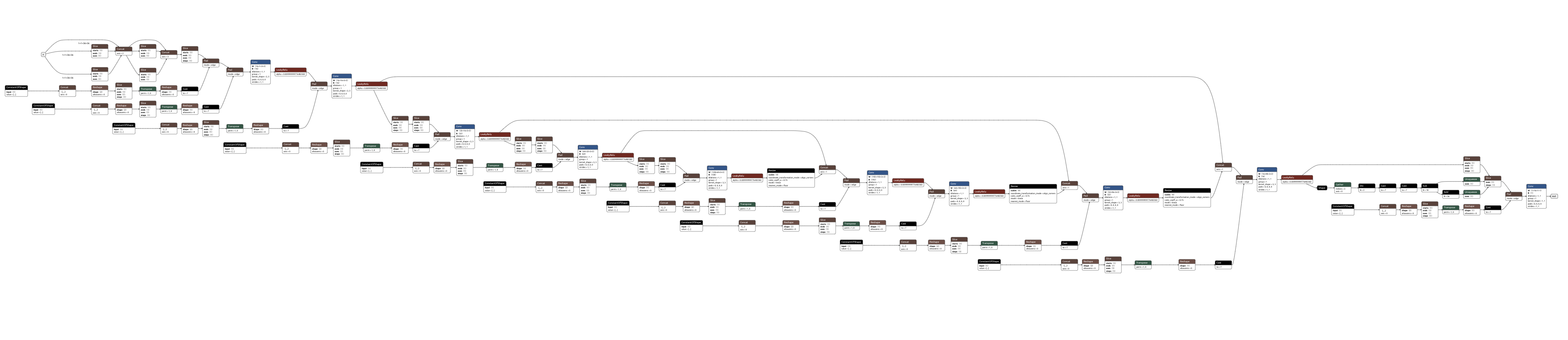
52	71%	[4, 2]	1	[2, 4]	16	219k params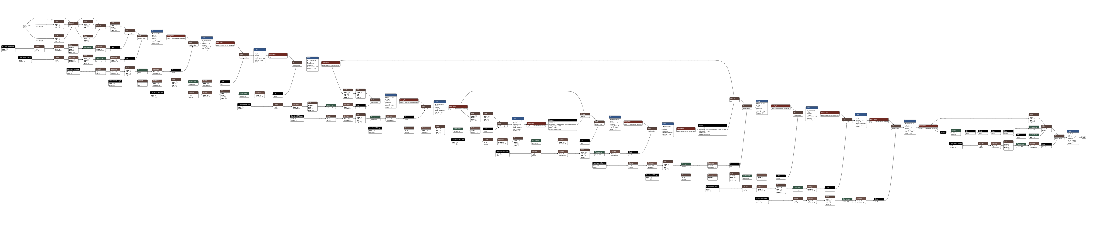

Note that the architecture defined in exp 2001 (with 576k parameters) performances will be boosted to 79% dice score to when trained with distillation (exp 1004).

The more the merrier... more parameters and larger architectures lead to better performances

Training¶

Defining experiments¶

An experiment is defined by as specific ID (like 300) and the whole configuration is versioned under git in the experiments_definition.py file:
- architecture (model name, number of layers, convolution sizes)
- augmentations
- loss (BCE, 🆕 BCE+Dice, BCE with more weights to the positive samples).
- hyper parameters
- distillation parameters (teacher is just the ID of a previous experiment, temperature, weight between distillation loss and label loss) 🆕
Tracking is performed using Weights and Biases see the dashboard here

Infrastructure¶

It is possible to train some experiments locally with a Nvidia very tiny GPU T500 with 4Gb of RAM.
- python TP_5/train.py -e 53 10
- -nowb allows disabling logging to weights and biases for quick prototyping
- -e to specify a list of experiments.
The same experiment can be trained on a remote server python TP_5/remote_training.py -e 53 10 -u kaggle_username -p
To be able to train on the remote servers of Kaggle with 16Gb of RAM, I customized a remote training template that I wrote (MVA-Pepites). I hosted the dataset under Kaggle. It is possible to train several experiments sequentially. More details here : remote training

Monitoring¶

I implemented a set of metrics on the validation set:

Accuracy (does not mean much because if the network returns all zeros, the accuracy is around 89%).
Precision , Recall. Recall seems interesting allows having a metric of how well we detected positive areas.
Segmentation specific metrics : Dice loss (also named F1-score) to measure the balance between precision and recall.
IoU (intersection over union).

🆕 We train the network using ~~BCE loss (with logits)~~ a combination of the Dice loss and BCE loss.

The problem is casted as a per-pixel binary classification (background = 0, foreground = 1). Since the background class is over represented, we can weight the positive class a bit more. The loss.py file shows the possibilities.

The best model selection is performed on the accuracy criterion (legacy)
The learning rate plateau decision is performed on the validation loss.

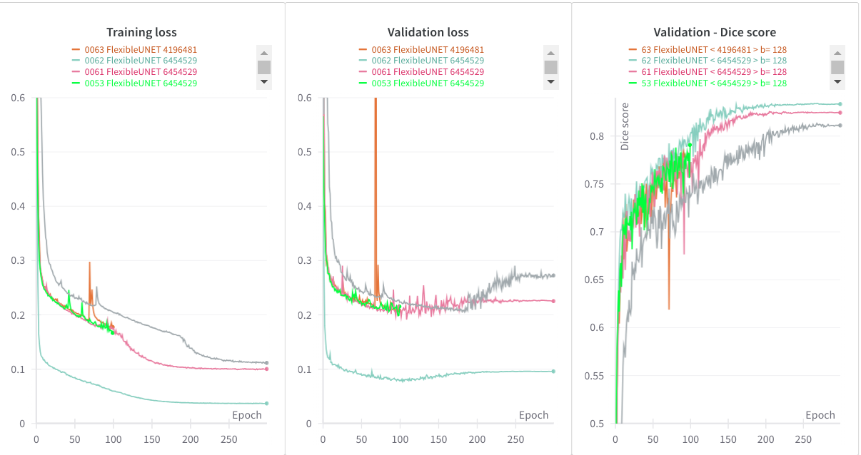
Training curves analyzis¶

Searching for the best architecture and hyper parameters¶

Below we exhibit all tests which have been performed (various archicture, sizes and several experiment to check hyper parameters)

Dice validation score

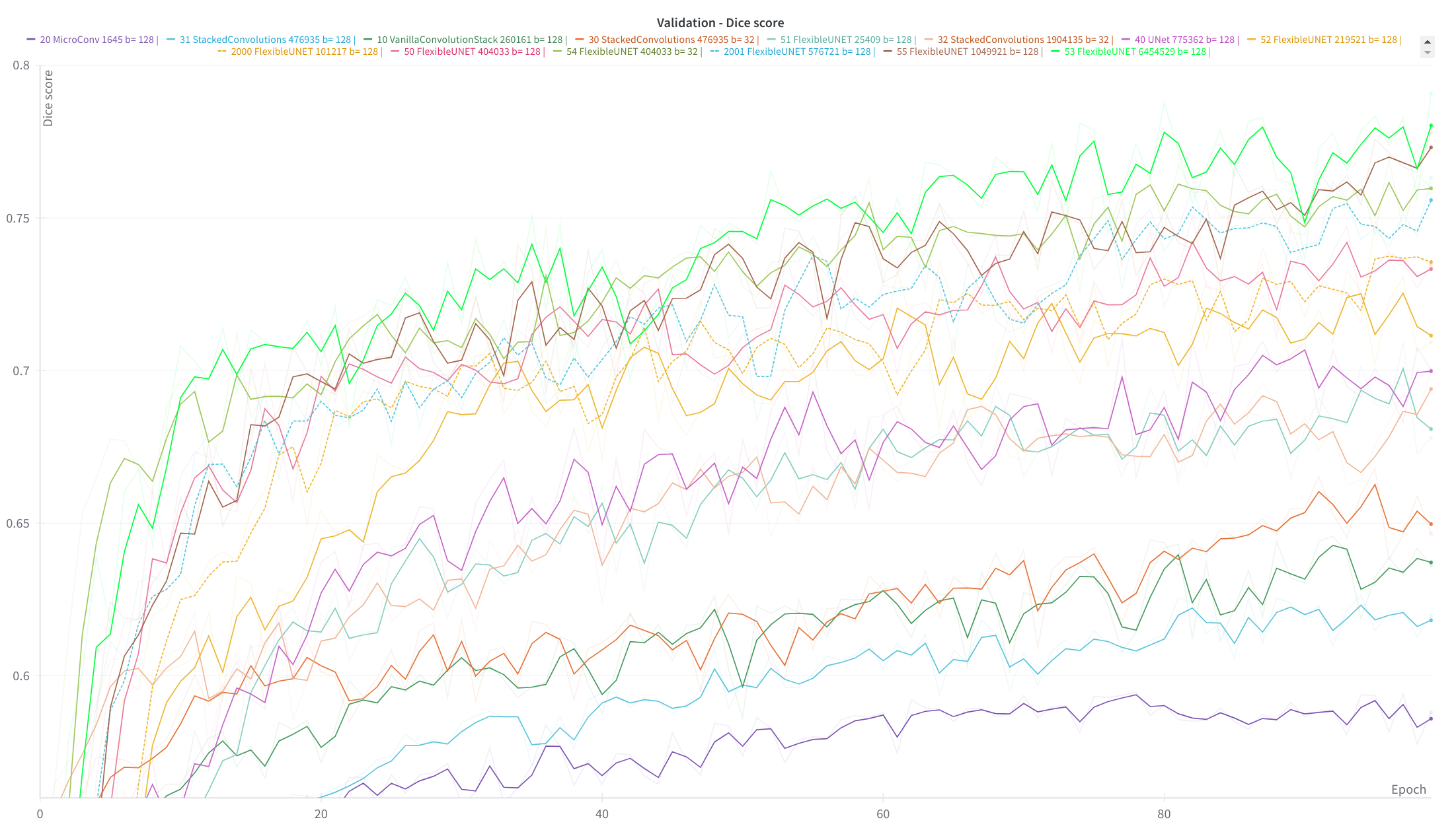Experiments configurations summary

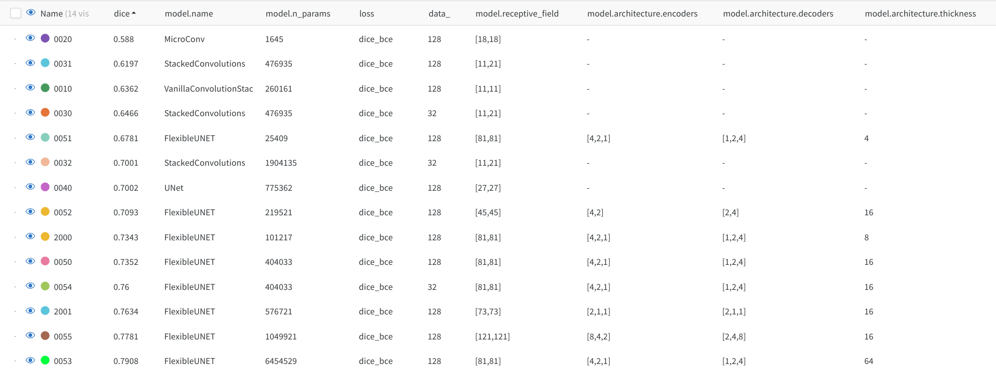Best model (teacher)¶

Experiment 53 .

Flexible UNET
3 scales, encoder [4, 2, 1] - bottleneck 1 - decoder [1, 2, 4]. Convolution block thickness 16, Leaky Relu.
Circular padding
6.4M parameters.
Adam Optimizer Learning rate LR $5 10^{-4}$ plateau (patience 10 epochs, LR decrease factor : $0.8$)
Stopped after 100 epochs before models start to overfit.
Augmentation: Horizontal shifts, vertical and horizontal flips.
Batch size 128

Overfitting for UNet with more than 4 million parameters.¶

Can we push this model further?

If you let the "big" networks train longer, we nottice that these end up overfitting (in the sense that training loss decreases and validation increases... while the dice loss we monitor remains kind of constant.)

The spotted overfitting truly affects the generalization capability of the model, making it go from 62% score to 58% on the challenge test set.

Note: I didn't have time to implement extra augmentations such as

exposure variation
S-curves
gaussian noise addition
geometric shear or tiny vertical rescales.

But I'm not sure that these extra augmentations or weight decay would be enough to prevent overfitting.

Results visualization¶

Batch inference¶

python TP_5/infer.py -e 1004 -m validation -o TP_5/__pretrained_models

Interactive visualization¶

To be able to visualize results, it is possible to perform live inference and compare several models. Inference is performed live on the GPU


We can browse between images using the left / right arrow	page up/ page down to switch between models	test mode without label

python TP_5/interactive_inference.py -i "TP_5/data/train/images/well_2*.npy" -e 53 1004 -m TP_5/pretrained_models --gui qt --preload

Using the right regexp, in the -i argument, you can select training, validation or test images.
Pretrained models (53 UNet6.4k, 1004 UNet 576k parameters) are provided.

Results analyzis¶

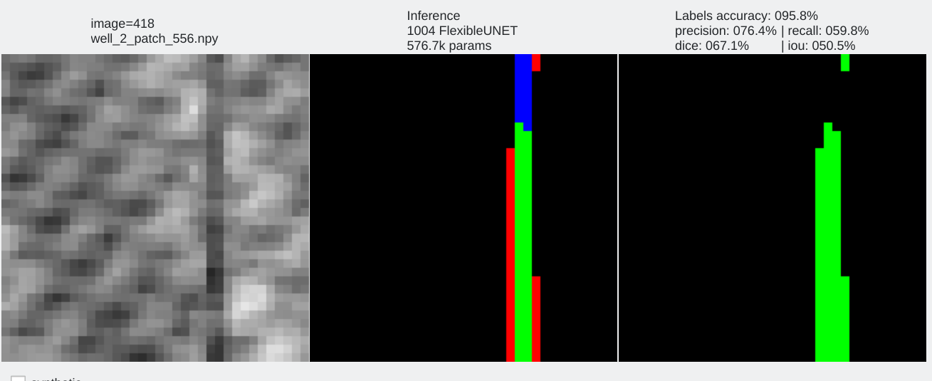
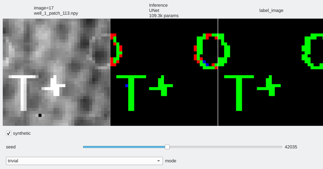
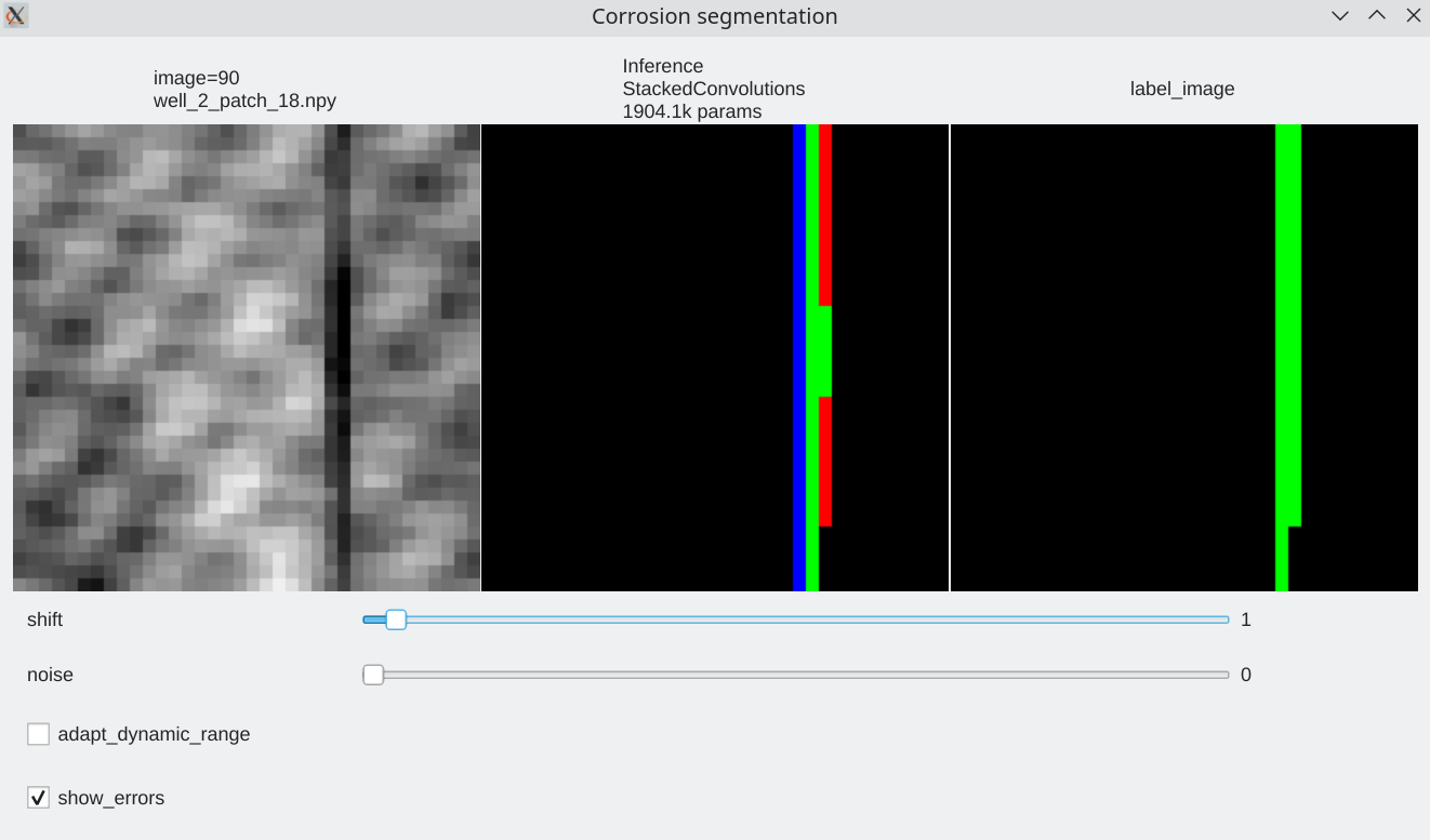
Color code¶

Pixels flagged in black or green: correctly labeled (black=background, green=foreground)
Pixels flagged in red: predicted background (0), groundtruth = foreground (1) a.k.a False Negative
Pixels flagged in blue: predicted foreground (1), groundtruth = background (0) a.k.a False Positive

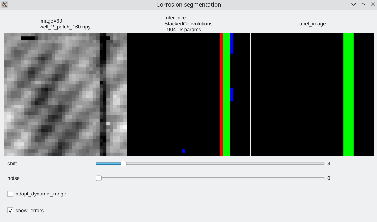
Coherence with shift and additive noise¶

Our stacked convolution network which uses horizontal convolutions with circular wrapping is able to segment corrosion areas which are located at the image boundary.
Segmentation results are almost unaffected by additive noise


Slider allow to shift the input horizontally	Slider allows to add a bit of noise

Labeling relevance¶

Trying to reach best accuracy may be in vain. As a matter of fact, it seems that sometimes the labels are less relevant than the network prediction.


Label mis-location	Label is too thick. Network prediction is more thin and better located. The corrosion line is 2 pixels wide , not 3

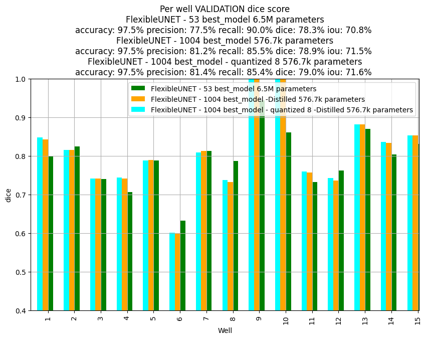
Making the model lightweight¶

Feel free to read the Weights and biases report on compressing the model

The following figures shows that performances remain equivalent with a huge reduction of model size and storage footprint (25MB teacher -> 550kb student + 8bits quantization).

Distillation¶

🔎 Weights and biases report section on distillation

Distillation has been added to the main training without the need to rewrite the whole code. We distilled the best model we got 53 UNET 6.4M parameters into a smaller 564k model (1004) which achieves similar performances.

Weights quantization¶

🔎 Weights and biases report section on quantization

Auxiliary notebook on quantization | code: model_quantization.ipynb

🪶 We'll use distilled model 1004 (UNET 564k) at first which weights 2.2Mb on disk as storing only 1.9M parameters.

We can quantify the weights to any precision we'd like 16bits or 8bits.
But we can try 12 or 4bits which would require a dedicated packing algorithm.

Weight quantization purpose is just to compress storage space (not RAM) at the cost of decompressing the weights. Not that lossless zip-like compression could be applied on top of that).

Remarks¶

Below is the global distribution of convolution weights of the model, no distinction made between layers.

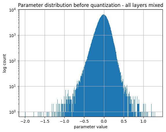
By analyzing the distribution of weights at each layer, it is clear that each layer's weight has its own range of values which is why I picked to quantify per layer.

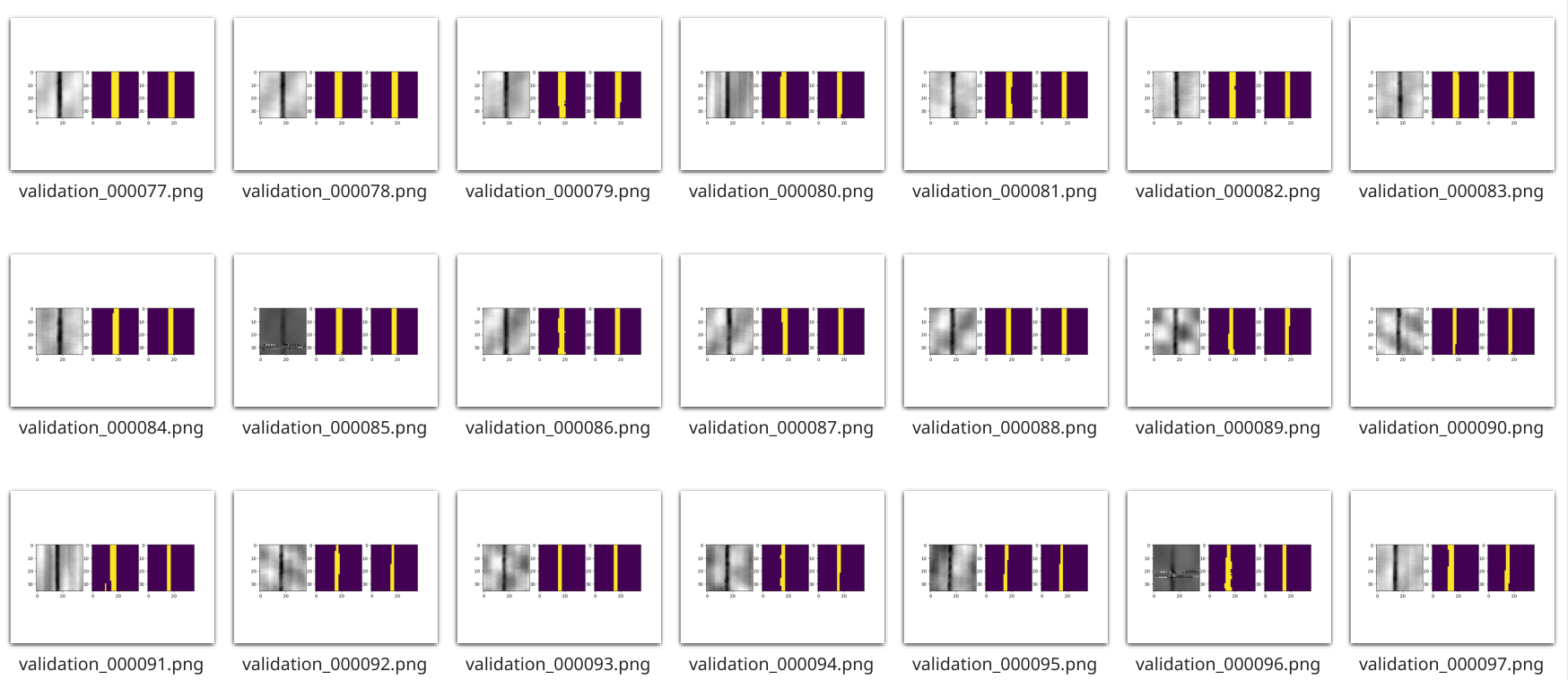
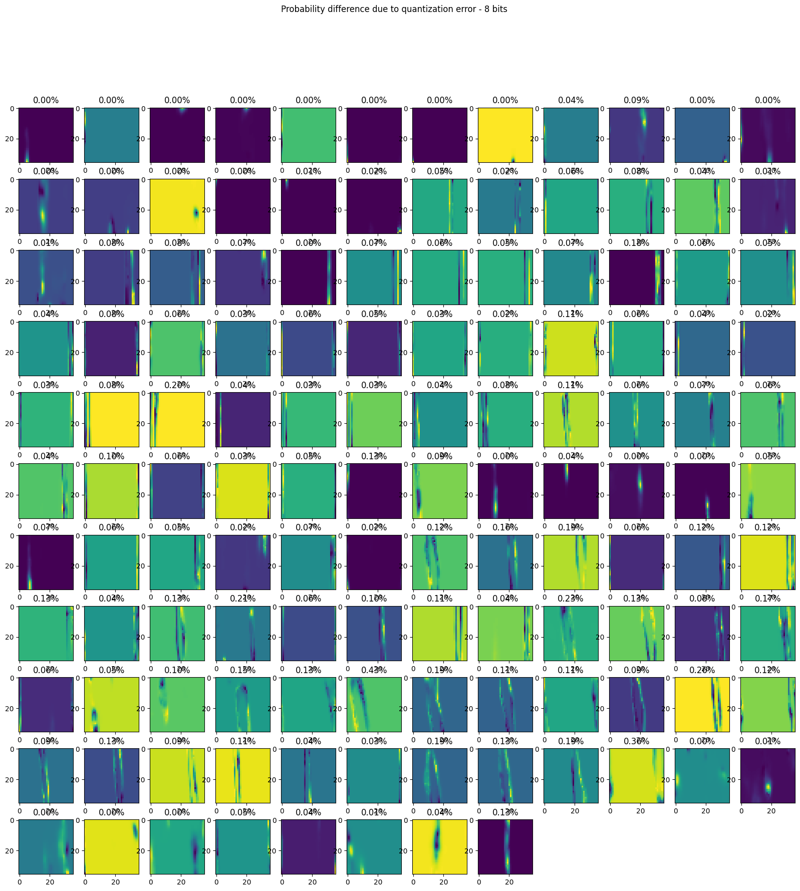
By compressing to signed 8bit integer weights, we're able to shrink the model by a factor of 4. If we take a look at the probability prediction errors with the 8bit compressed model, we have a less than an average 0.1% error and visually the segmentations prediction with the quantized weights don't look to far away from the original model. We can check the first validation batch (128 images).

Here's the summary on performances of quantization of model 1004.

Quantization	None	16bits	8bits	4bits
Size on disk	2.2MB	1.1MB	550kB	$\leq$ 300kB
Format	Float32	int16	int8	packed 1 bit of sign + 3bits content
Dice Score	78.937%	78.95%	78.956%	73.41%
IoU	71.549%	71.57%	71.584%	65.15%
Dice score test set	66.24%	-	66.38%	-

Conclusion¶

This project was an interesting first contact with segmentation and model compression.

The design of a UNet tailored for the specificities of well imaging (circular azimuth, and very small 36x36) has allowed to achieve correct performances at segmenting corroded areas.
It is possible to shrink the segmentation model down to a point where it can be stored on 550kB (for instance as part of the firmware binary).
Generalization capabilities to unseen wells are probably not so great (as reflected by the score on the data challenge - I achieved a maximum of 66.24% score)...

Test set score: 66.24

Limitations and potential improvements¶

A lot of time during this project was spent on the "reboot" phase to find and correct a few issues mentioned at the begining.

Potential improvements¶

Here are some ideas for improvements:

One important point is that we only have access to a tiny vertical windows and I guess that the relevance could be much improved if we'd treat larger vertical windows (corrosion areas seem to often look a lot like dark lines). Taking decisions near the vertical boundaries of the 36x36 image is much harder when you don't have a clue what's above or below.
An ensembling technique could have been deployed (majority voting between several models)...to be later distilled into a smaller model.
Hard Negative Mining: Once we get a first network, we could mine the difficult examples (evaluate the performances over all patches and sort the most difficult ones). In a second step, we can re-train the pretrained network on these hard patches.
About the UNet architecture: Max pooling could have been used (instead of skipping) and stride convolutions instead of bilinear upsampling. Same goes with batch normalization.
A simple review of the predicted mask sometimes reveal a few isolated unlikely pixels... A few morphological operations like closing/opening could aleviate a few false positives.

Missing elements¶

Due to the time spent on the TP-5 lab session and project, here are some points I didn't have time to implement.

~~"Dice Loss Bug": For some reason, I could not minimize the dice loss (1-dice coefficient). Don't know whether the loss is wrong or not.~~ -> fixed
Extra augmentation by a bit of additive white gaussian noise, blur or sharpening, multiply the signals to slightly augment the dynamic range, add S curves to augment (increase/decrease contrast).
~~perform an evaluation of the metrics per well (there may be more difficult wells).~~
try the so called Focal Loss which is said to adapt the weight of the BCE kind of automatically.
cross validation (take several split of the train, validation set and evaluate the average and standard deviation of the results for 1 experiment configuration). Could have been interesting to check generalization capabilities to totally unseen wells.
(Not asked) effort to reduce the model memory footprint in RAM or execution time assessment
Label refinement: questioning the quality of the dataset and labels is important but improving it (either automatically or semi-automatically) is a huge task and moreover, we don't play a fair game here as we only have 36x36 patches (and sometimes corrosion is hard to see to the naked eye honnestly - i think the annotations have been made with a full vision of the well, coherence along the vertical axis may have helped annotators a lot).

True difficulties¶

Very difficult to assess the quality of annotations. -> A toy example has been made to make sure everything was ok.
~~Not sure whether or not the validation loss starts increasing because of overfitting or basically that the validation set does not have the same distribution as the training set!~~ -> Re-done dataset split.